


Jet Reports, often referred to simply as “Jet,” is a reporting and analytics tool for Microsoft Dynamics Navision (NAV), an enterprise resource planning solution. Jet functions as a Microsoft Excel add-in that allows users to access NAV data quickly to create ad-hoc reports. Since Jet is specifically designed for the Microsoft Dynamics product suite, it provides more flexibility for users when creating NAV reports than other more competitive data-visualization tools. With an intuitive user interface and pre-built data model, Jet Reports is an easy self-service tool for quick-to-market NAV reports designed by business users who don’t necessarily have data modeling experience.
On a recent project, I developed operational and management reports within Jet as part of a Microsoft NAV implementation for a manufacturing company, and I’ve developed a short list of tips to get the most out of the tool. Jet has an online community and knowledge base, but I felt it would be helpful to provide an additional resource by listing solutions to three challenges I faced.
Tip 1: Referencing Cells in a Jet Grouping
While developing reports, I often found myself working within a grouping that needs to reference a cell outside of that grouping. Because the default Jet functionality is to expand rows downward upon running, it becomes difficult to know exactly what cell to reference to get the needed data. The following cell reference work around is a method I’ve used to solve this issue in countless reports. This approach is essential if you have multiple groupings where each subsequent grouping references an earlier grouping.
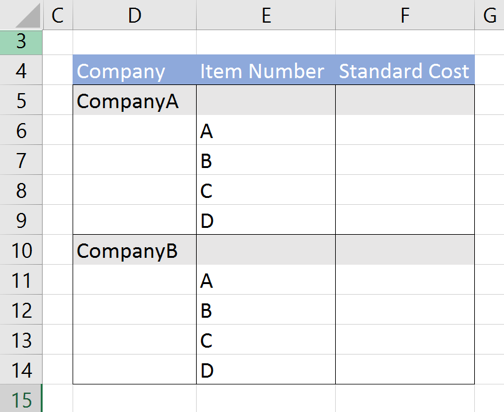
Suppose you’re pulling a distinct list of companies from NAV, along with the item numbers and corresponding cost for each.
After launching Jet, list out all companies by writing an NL(“Rows”) statement against the Item table in cell D5 of your workbook.
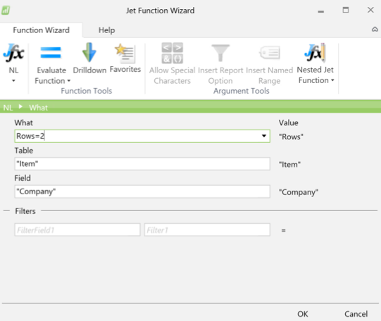

Note: The “What” parameter will be Rows = 2 because another NL(“Rows”) statement will be used within your Rows statement.
Next, to list out all items per company, write an NL(“Rows”) statement below the previous statement, referencing the company (cell E6).
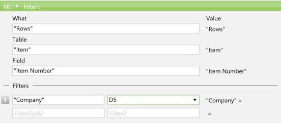
Each item should be listed by company. Now, let’s get into the cell reference workaround.
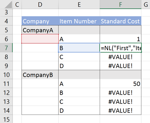
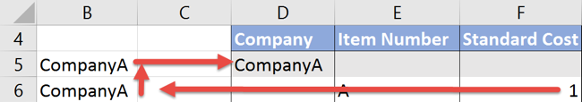
To look up the standard cost for items by company, write an NL(“First”) statement in cell F6 referencing the Item Number and Company. By referencing the Company from cell D5 (up one cell and to the left two cells), the first item number is displayed correctly. Unfortunately, when the NL(“Rows”) function expands for the remaining item numbers, the next NL(“First”) statement (cell F7) will continue to evaluate up one cell and over two to the left. This will reference a blank field for every row except the first. As shown below, an error is displayed for the remaining rows when using this approach:
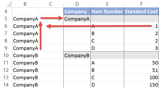
To eliminate this error, reference the company cell from a hidden column to the left in the same row as the initial NL(“Rows”) statement (cell D5 in this example). For this example, column B will be used. In every cell below B5, reference the cell above it all the way through to when the Company reference is needed. When Jet expands the report, the workaround column will expand with it. Reference the hidden Company column for Company in the Standard Cost field (cell F6), as shown below.
This allows you to reference the company from anywhere in that grouping. When the report is run, your results should include the appropriate data without any errors.
Tip 2: Filtering Rows Based on Inequality of Two Columns
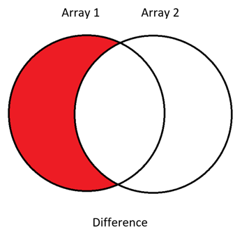
Another common scenario I faced was the need to compare two columns from two different tables and only display the rows where these two columns did not match. An initial solution was to bring in all rows and do a conditional hide on rows where the columns did match. This works, but if 99% of the two columns match, this isn’t going to be an efficient approach. A more effective solution is to use the NL(“Filter”) function to create lists of values along with the NL(“Difference”) function over these arrays to return the desired list of values. NL(“Difference”) takes in two NL(“Filter”) formulas, Array 1 and Array 2, with the result being all items in Array 1 that are not in Array 2, as shown in the following diagram:
Note: For this method to work, you must be able to identify every row in the input table with a non-composite primary key. This is because arrays in Jet can only hold a single value, a value later used to identify the row in the dataset.
Array 1 will be all keys from the desired output table, and Array 2 will be all keys from this table where the two columns being compared are the same (these arrays are created using NL(“Filter”)). The comparison between the two columns in Array 2 is done by using a “Link=” function with the two columns in question as the links (in addition to any links normally required to join the two tables). This link will remove any records where the two columns in question do not match. With Array 1 and Array 2 as inputs to the NL(“Difference”), the result is a list of all keys where the two columns do not match.
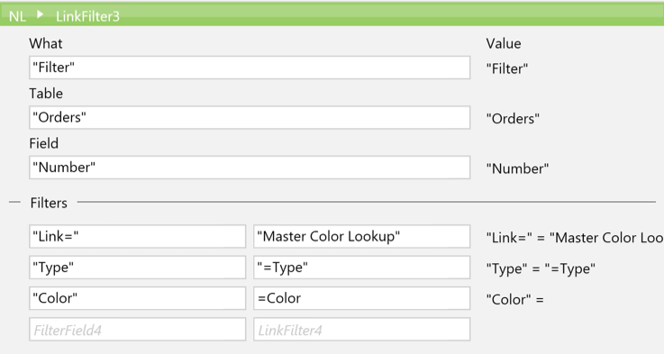
For example, start with a table containing a list of orders (the non-composite primary key). Each row has an Order Number, a Type, and a Color to make the order in (e.g., (Order Number: 001, Type: Pencil, Color: Blue)). Another table exists that is a list of the standard color that should go with each type (e.g., (Type: Pencil, Color: Blue), (Type: Pen, Color: Red), (Type: Stapler, Color: Black)). The goal is to list all orders where the color in the order does not match that of the standard color table. To begin, the first array (cell C2) is as follows:
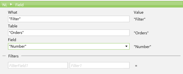
This NL(“Filter”) will give a list of all Numbers from the Order table. The second array is all Numbers in the Order table with a matching color as that in the Master Color Lookup. The “Link=” is where rows having a Type and Color that do not match will be eliminated.
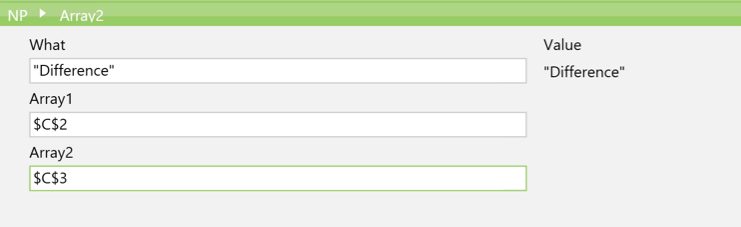
If we do an NP(“Difference”) function over these two filters, we will achieve the correct result. The result is all orders that appeared in Array 1 (all items from our orders list) minus all items that appeared in Array 2 (all items where the color matches the standard color), giving us a result of all items where the color does not match the standard color.
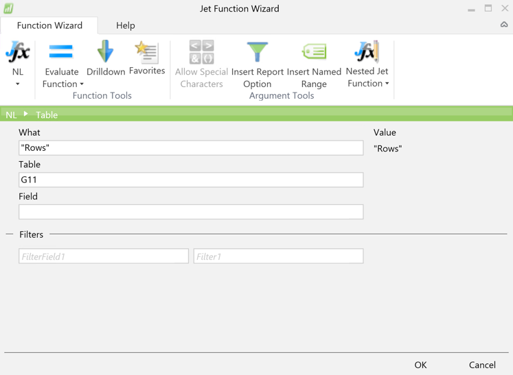
This NP(“Difference”) can be used in an NL(“Rows”) statement as the “Table” parameter to list out all keys in the NP(“Difference”) array. For this example, assume the NL(“Difference”) array is in cell G11. The resulting NL(“Rows”) statement would appear as follows:
Tip 3: SQL= as an Alternative
Lastly, we have what I believe to be the most powerful feature in Jet: SQL=. Because Jet Reports is an Excel add-in and doesn’t integrate SQL queries beyond this function, some reporting requirements may be more difficult than others to build. SQL= allows users to create a table using a SQL statement from which data for the report can be pulled. I personally prefer to only use SQL= in my reports as a last resort because, while it is very efficient, I believe utilizing Jet functionality to build my reports yields a sleeker and easier to understand product for anybody else viewing the reports.
For example, assume the objective is to list all “No” from the Posted Sales Transactions where the sum of the Quantity over all “No” is greater than zero, grouped by Company and for only “Company A”. Also, assume that the Company is determined by a user input at run-time. A %Filter% statement is needed in the SQL= statement to apply this filter. The format for a SQL= statement is the concatenation of the string “SQL=” and the SQL statement needed to pull the data:

This statement can be used as the “Table” parameter in an NL(“Rows”) statement to pull all values with the applied filters. In general, the SQL= statement can return any number of fields from any number of tables. Like in SQL, if there are ambiguous columns between tables, aliasing can be used in the SQL statement to make the distinction. With aliasing, the same SQL statement would appear as such:

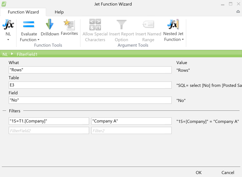
If this statement is placed in cell E3, the following NL(“Rows”) statement will correctly pull back all “No” that have a total Quantity greater than zero. Note the syntax for the Filter Field is “1S=T1.[Company]”. The ‘1’ corresponds to the Filter number in the report, the ‘S’ indicates that the value being pulled back is a String (versus a Number ‘N’ or Date ‘D’), and T1.[Company] is the column that is being filtered on in the statement.
Note: The Jet Drilldown functionality cannot be used in data sets that result from SQL=. Additionally, SQL= is not available for live connections directly against NAV.
Follow-up Questions
If your company is wondering how to put these tips into practice, feel free reach out to us at marketing@credera.com. We’d love to help as you think through how your company can gain valuable insights through reporting and analytics.
Contact Us
Let's talk!
We're ready to help turn your biggest challenges into your biggest advantages.
Searching for a new career?
View job openings